Backtrack
Overview
The backtrack module is used to find paleo water depths from a tectonic subsidence model, and sediment decompaction over time.
The tectonic subsidence model is either an age-to-depth curve (in ocean basins) or rifting (near continental passive margins).
Running backtrack
You can either run backtrack as a built-in script, specifying parameters as command-line options (...):
python -m pybacktrack.backtrack_cli ...
…or import pybacktrack into your own script, calling its functions and specifying parameters as function arguments (...):
import pybacktrack

pybacktrack.backtrack_and_write_well(...)
Note
You can run python -m pybacktrack.backtrack_cli --help to see a description of all command-line options available, or
see the backtracking reference section for documentation on the function parameters.
Example
For example, revisiting our backtracking example, we can run it from the command-line as:
python -m pybacktrack.backtrack_cli \
    -w pybacktrack_examples/example_data/ODP-114-699-Lithology.txt \
    -d age compacted_depth compacted_thickness decompacted_thickness decompacted_density decompacted_sediment_rate decompacted_depth dynamic_topography water_depth tectonic_subsidence paleo_longitude paleo_latitude compacted_density composite_porosity composite_decay lithology \
    -ym M2 \
    -slm Haq87_SealevelCurve_Longterm \
    -o ODP-114-699_backtrack_amended.txt \
    -- \
    ODP-114-699_backtrack_decompacted.txt
…or write some Python code to do the same thing:
import pybacktrack

# Input and output filenames.
input_well_filename = 'pybacktrack_examples/example_data/ODP-114-699-Lithology.txt'
amended_well_output_filename = 'ODP-114-699_backtrack_amended.txt'
decompacted_output_filename = 'ODP-114-699_backtrack_decompacted.txt'

# Read input well file, and write amended well and decompacted results to output files.
pybacktrack.backtrack_and_write_well(
    decompacted_output_filename,
    input_well_filename,
    dynamic_topography_model='M2',
    sea_level_model='Haq87_SealevelCurve_Longterm',
    # The columns in decompacted output file...
    decompacted_columns=[pybacktrack.BACKTRACK_COLUMN_AGE,
                         pybacktrack.BACKTRACK_COLUMN_COMPACTED_DEPTH,
                         pybacktrack.BACKTRACK_COLUMN_COMPACTED_THICKNESS,
                         pybacktrack.BACKTRACK_COLUMN_DECOMPACTED_THICKNESS,
                         pybacktrack.BACKTRACK_COLUMN_DECOMPACTED_DENSITY,
                         pybacktrack.BACKTRACK_COLUMN_DECOMPACTED_SEDIMENT_RATE,
                         pybacktrack.BACKTRACK_COLUMN_DECOMPACTED_DEPTH,
                         pybacktrack.BACKTRACK_COLUMN_DYNAMIC_TOPOGRAPHY,
                         pybacktrack.BACKTRACK_COLUMN_WATER_DEPTH,
                         pybacktrack.BACKTRACK_COLUMN_TECTONIC_SUBSIDENCE,
                         pybacktrack.BACKTRACK_COLUMN_SEA_LEVEL,
                         pybacktrack.BACKTRACK_COLUMN_PALEO_LONGITUDE,
                         pybacktrack.BACKTRACK_COLUMN_PALEO_LATITUDE,
                         pybacktrack.BACKTRACK_COLUMN_COMPACTED_DENSITY,
                         pybacktrack.BACKTRACK_COLUMN_COMPOSITE_POROSITY,
                         pybacktrack.BACKTRACK_COLUMN_COMPOSITE_DECAY,
                         pybacktrack.BACKTRACK_COLUMN_LITHOLOGY],
    # Might be an extra stratigraphic well layer added from well bottom to basement...
    ammended_well_output_filename=amended_well_output_filename)
Note
The drill site file pybacktrack_examples/example_data/ODP-114-699-Lithology.txt is part of the example data.
Backtrack output
For each stratigraphic layer in the input drill site file, backtrack can write one or more parameters to an output file.
Running the above example on ODP drill site 699:
# SiteLongitude = -30.677
# SiteLatitude = -51.542
# SurfaceAge = 0

## bottom_age bottom_depth lithology
   18.7       85.7         Diatomite 0.7 Clay 0.3
   25.0       142.0        Coccolith_ooze 0.3 Diatomite 0.5 Mud 0.2
   31.3       233.6        Coccolith_ooze 0.3 Diatomite 0.7
   31.9       243.1        Sand 1
   36.7       335.4        Coccolith_ooze 0.8 Diatomite 0.2
   40.8       382.6        Chalk 1
   54.5       496.6        Chalk 1
   55.3       516.3        Chalk 0.5 Clay 0.5
…produces an amended drill site output file containing an extra base sediment layer, and a decompacted output file containing the decompacted output parameters like sediment thickness and water depth.
Amended drill site output
The amended drill site output file:
# SiteLatitude = -51.5420
# SiteLongitude = -30.6770
# SurfaceAge = 0.0000
#
## bottom_age bottom_depth lithology
   18.700     85.700       Diatomite       0.70       Clay            0.30
   25.000     142.000      Coccolith_ooze  0.30       Diatomite       0.50       Mud             0.20
   31.300     233.600      Coccolith_ooze  0.30       Diatomite       0.70
   31.900     243.100      Sand            1.00
   36.700     335.400      Coccolith_ooze  0.80       Diatomite       0.20
   40.800     382.600      Chalk           1.00
   54.500     496.600      Chalk           1.00
   55.300     516.300      Chalk           0.50       Clay            0.50
   79.133     601.000      Shale           1.00
There is an extra base sediment layer that extends from the bottom of the drill site (516.3 metres) to the total sediment thickness (601 metres). The bottom age of this new base layer (79.133 Ma) is the age of oceanic crust that ODP drill site 699 is on. If it had been on continental crust (near a passive margin such as DSDP drill site 327) then the bottom age of this new base layer would have been when rifting started (since we would have assumed deposition began when continental stretching began).
Decompacted output
The decompacted output file:
# SiteLatitude = -51.5420
# SiteLongitude = -30.6770
# SurfaceAge = 0.0000
#
# age       compacted_depth compacted_thickness decompacted_thickness decompacted_density decompacted_sediment_rate decompacted_depth dynamic_topography water_depth tectonic_subsidence sea_level paleo_longitude paleo_latitude compacted_density composite_porosity composite_decay lithology
  0.000     0.000           601.000             601.000               1726.994            5.810                     0.000             0.000              3798.317    4134.284            57.262    -30.677         -51.542        2540.400          0.816              680.800         Diatomite       0.70       Clay            0.30
  18.700    85.700          515.300             552.679               1733.298            10.682                    108.648           75.174             3604.761    3872.267            80.240    -25.677         -51.447        2529.100          0.669              1119.000        Coccolith_ooze  0.30       Diatomite       0.50       Mud             0.20
  25.000    142.000         459.000             518.231               1715.612            24.388                    175.945           88.541             3543.441    3770.680            94.287    -23.719         -51.519        2532.900          0.765              803.200         Coccolith_ooze  0.30       Diatomite       0.70
  31.300    233.600         367.400             431.443               1727.755            16.781                    329.587           102.254            3536.973    3651.861            128.239   -21.447         -51.598        2650.000          0.490              3704.000        Sand            1.00
  31.900    243.100         357.900             424.770               1719.132            25.543                    339.656           104.005            3544.482    3639.106            140.124   -21.230         -51.601        2659.400          0.640              1415.200        Coccolith_ooze  0.80       Diatomite       0.20
  36.700    335.400         265.600             342.298               1675.058            17.557                    462.265           128.465            3467.220    3519.684            133.878   -19.707         -51.659        2710.000          0.700              1408.000        Chalk           1.00
  40.800    382.600         218.400             291.817               1662.325            13.524                    534.247           133.268            3439.494    3423.104            157.463   -18.675         -51.706        2710.000          0.700              1408.000        Chalk           1.00
  54.500    496.600         104.400             147.135               1649.440            45.709                    719.529           161.651            3103.703    2999.804            146.017   -16.433         -52.672        2722.500          0.730              1330.000        Chalk           0.50       Clay            0.50
  55.300    516.300         84.700              114.840               1678.129            5.054                     756.096           162.953            3116.404    2970.460            157.769   -16.239         -52.750        2700.000          0.630              1960.000        Shale           1.00
The age, compacted_depth and lithology columns are the same as the bottom_age, bottom_depth and lithology columns in the input drill site (except there is also a row associated with the surface age).
The compacted_thickness column is the total sediment thickness (601 metres - see base sediment layer of amended drill site above) minus compacted_depth. The decompacted_thickness column is the thickness of all sediment at the associated age. In other words, at each consecutive age another stratigraphic layer is essentially removed, allowing the underlying layers to expand (due to their porosity). At present day (or the surface age) the decompacted thickness is just the compacted thickness. The decompacted_density column is the average density integrated over the decompacted thickness of the drill site (each stratigraphic layer contains a mixture of water and sediment according to its porosity at the decompacted depth of the layer). The decompacted_sediment_rate column is the rate of sediment deposition in units of metres/Ma. At each time it is calculated as the fully decompacted thickness (ie, using surface porosity only) of the surface stratigraphic layer (whose deposition ends at the specified time) divided by the layer’s deposition time interval. The decompacted_depth column is similar to decompacted_sediment_rate in that the stratigraphic layers are fully decompacted (using surface porosity only) as if no portion of any layer had ever been buried. It is also similar to compacted_depth except all effects of compaction have been removed.
The dynamic_topography column is the dynamic topography elevation relative to present day (or zero if no dynamic topography model was specified). The tectonic_subsidence column is the output of the underlying tectonic subsidence model, and water_depth is obtained from tectonic subsidence by subtracting an isostatic correction of the decompacted sediment thickness.
The paleo_longitude and paleo_latitude columns contain the paleo location of the drill site at each age.
Finally, the compacted_density, composite_porosity and composite_decay columns contain the density, porosity and porosity decay of the stratigraphic layer (whose deposition ends at the specified time). And since a single stratigraphic layer can have a mixture of weighted lithologies, these three values represent the density, porosity and porosity decay of the final lithology (weighted combination of mixture lithologies). Also note that compacted_density is just for a single stratigraphic layer, unlike decompacted_density which is an average density over multiple decompacted layers.
Note
The output columns are specified using the -d command-line option (run python -m pybacktrack.backtrack_cli --help to see all options), or
using the decompacted_columns argument of the pybacktrack.backtrack_and_write_well() function.
By default, only age and decompacted_thickness are output.
By default, the rows are associated with the stratigraphic ages in the input drill site.
However, you can specify your own time for each row using the -tl or -tr command-line options (run python -m pybacktrack.backtrack_cli --help for more details)
or using the times argument of the pybacktrack.backtrack_and_write_well() function.
And it’s OK to specify times that are outside the period of sediment deposition recorded in the drill site
(eg, older than the drill site’s bottom age or younger than its surface age). You will still get rows for these times.
Note
Specifying your own times (eg, using -tl or -tr command-line options) means that a time could fall inside a stratigraphic unit
(ie, not exactly on a stratigraphic boundary, as in the default case).
In this case, a sub-section of the surface stratigraphic unit (that’s at the surface at the specified time) is stripped off to create a
partial unit.
The part that’s stripped off is from the unit’s top age to the specified time (assuming a constant sediment deposition rate for the unit).
Paleo locations of drill site
The present day location of a drill site is assigned a plate ID and reconstructed back through time (using a reconstruction model consisting of static polygons and rotations). The reconstructed locations at each stratigrahic age become the paleo_longitude and paleo_latitude columns of the decompacted output file.
You can either use the default built-in reconstruction model, or specify your own static polygon and rotation files
(using the --static_polygon_filename and --rotation_filenames command-line options).
The default reconstruction model is Zahirovic 2022:
Zahirovic, S., Eleish, A., Doss, S., Pall, J., Cannon, J., Pistone, M., Tetley, M. G., Young, A., & Fox, P. (2022), Subduction kinematics and carbonate platform interactions. Geoscience Data Journal, 9(2), p.371-383, (data obtained here)
The default reference frame for the Zahirovic 2022 model is the mantle reference frame (anchor plate 0).
Alternatively you can use its paleomagnetic reference frame by specifying anchor plate 701701 (using the command-line option --anchor 701701).
This can be useful for paleoclimate-related research.
Note
Sea level variation
A model of the variation of sea level relative to present day can optionally be used when backtracking. This adjusts the isostatic correction of the decompacted sediment thickness to take into account sea-level variations.
These are the built-in sea level models bundled inside backtrack:
Miller2024_SealevelCurve- Global Mean and Relative Sea-Level Changes Over the Past 66 Myr: Implications for Early Eocene Ice SheetsHaq2024_Hybrid_SealevelCurve- Combined Haq (2014) and Haq (2017) sea level curves for the Cretaceous and Jurassic respectively, with the Cenozoic section of Haq and Ogg (2024).0-66 Ma: Haq and Ogg (2024)
66-140 Ma: Haq (2014)
140.1-205 Ma: Haq (2017)
Haq2024_Hybrid_SealevelCurve_Longterm- Long-term curve.Note that while this is from Haq and Ogg (2024), it is digitized to follow the peaks of the shorter term curve.
Haq87_SealevelCurve- The Phanerozoic Record of Global Sea-Level ChangeHaq87_SealevelCurve_Longterm- Long-term curve.Normalised to start at zero at present-day.
A sea-level model is optional. If one is not specified then sea-level variation is assumed to be zero.
Note
A built-in sea-level model can be specified using the -slm command-line option (run python -m pybacktrack.backtrack_cli --help to see all options), or
using the sea_level_model argument of the pybacktrack.backtrack_and_write_well() function.
Note
It is also possible to specify your own sea-level model. This can be done by providing your own text file containing a column of ages (Ma) and a
corresponding column of sea levels (m), and specifying the name of this file to the -sl command-line option or to the sea_level_model argument
of the pybacktrack.backtrack_and_write_well() function.
Oceanic and continental tectonic subsidence
Tectonic subsidence is modelled separately for ocean basins and continental passive margins.
The subsidence model chosen by the backtrack module depends on whether the drill site is on oceanic or continental crust.
This is determined by an oceanic age grid. Since the age grid captures only oceanic crust, a drill site inside this region
will automatically use the oceanic subsidence model whereas a drill site outside this region uses the continental subsidence model.
The default present-day age grid bundled inside backtrack is a 6-minute resolution grid
of the age of the world’s ocean crust that uses the timescale of Gee and Kent (2007):
Seton, M., Müller, R. D., Zahirovic, S., Williams, S., Wright, N., Cannon, J., Whittaker, J., Matthews, K., McGirr, R., (2020), A global dataset of present-day oceanic crustal age and seafloor spreading parameters, Geochemistry, Geophysics, Geosystems, doi: 10.1029/2020GC009214
Note
The default present-day age grid was updated in pyBacktrack version 1.4.
Note
You can optionally specify your own age grid using the -a command-line option (run python -m pybacktrack.backtrack_cli --help to see all options), or
using the age_grid_filename argument of the pybacktrack.backtrack_and_write_well() function.
Oceanic versus continental drill sites
ODP drill site 699 is located on deeper ocean crust (as opposed to shallower continental crust):
# SiteLongitude = -30.677
# SiteLatitude = -51.542
# SurfaceAge = 0

## bottom_age bottom_depth lithology
   18.7       85.7         Diatomite 0.7 Clay 0.3
   25.0       142.0        Coccolith_ooze 0.3 Diatomite 0.5 Mud 0.2
   31.3       233.6        Coccolith_ooze 0.3 Diatomite 0.7
   31.9       243.1        Sand 1
   36.7       335.4        Coccolith_ooze 0.8 Diatomite 0.2
   40.8       382.6        Chalk 1
   54.5       496.6        Chalk 1
   55.3       516.3        Chalk 0.5 Clay 0.5
So it will use the oceanic subsidence model.
See also
In contrast, DSDP drill site 327 is located on shallower continental crust (as opposed to deeper ocean crust):
# SiteLongitude = -46.7837
# SiteLatitude = -50.8713
# RiftStartAge = 160
# RiftEndAge = 120
# SurfaceAge = 0

## bottom_age bottom_depth lithology
   1.5        10.0         Shaley_sand 1
   55.8       30.0         Clay 1
   59.9       68.0         Diatomite 0.7 Clay 0.3
   62.2       90.0         Clay 1
   77.4       142.0        Coccolith_ooze 0.7 Biogenic_sand 0.3
   86.4       154.0        Clay 1
   113.1      324.0        Coccolith_ooze 0.3 Clay 0.7
   122.3      469.5        Clay 1
So it will use the continental subsidence model. Since continental subsidence involves rifting, it requires a rift start and end time.
These extra rift parameters can be specified at the top of the drill site file as RiftStartAge and RiftEndAge attributes
(see Continental subsidence).
See also
If you are not sure whether your drill site lies on oceanic or continental crust then first prepare your drill site assuming it’s on
oceanic crust (since this does not need rift start and end ages). If an error message is generated when
running backtrack then you’ll need to determine the rift start and end age, then
add these to your drill site file as RiftStartAge and RiftEndAge attributes, and then run backtrack again.
Note
In pyBacktrack version 1.4 if the RiftStartAge and RiftEndAge attributes are not specified in your drill site file then
they are obtained implicitly from the built-in rift start/end time grids (see Continental subsidence), so an
error message is unlikely to be generated when your drill site file is on continental crust.
Present-day tectonic subsidence
The tectonic subsidence at present day is used in both the oceanic and continental subsidence models.
Tectonic subsidence is unloaded water depth, that is with sediment removed.
So to obtain an accurate value, backtrack starts with a bathymetry grid to obtain the present-day water depth (the depth of the sediment surface).
Then an isostatic correction of the present-day sediment thickness (at the drill site) takes into account the removal of sediment to reveal
the present-day tectonic subsidence. The isostatic correction uses the average sediment density of the drill site stratigraphy.
The default present-day bathymetry grid bundled inside backtrack is a
6-minute resolution global grid of the land topography and ocean bathymetry (although only the ocean bathymetry is actually needed):
Amante, C. and B. W. Eakins, ETOPO1 1 Arc-Minute Global Relief Model: Procedures, Data Sources and Analysis. NOAA Technical Memorandum NESDIS NGDC-24, 19 pp, March 2009
Note
You can optionally specify your own bathymetry grid using the -t command-line option (run python -m pybacktrack.backtrack_cli --help to see all options), or
using the topography_filename argument of the pybacktrack.backtrack_and_write_well() function.
Note
If you specify your own bathymetry grid, ensure that its ocean water depths are negative. It is assumed that elevations in the grid above/below sea level are positive/negative.
Oceanic subsidence
Oceanic subsidence is somewhat simpler and more accurately modelled than continental subsidence (due to no lithospheric stretching).
The age of oceanic crust at the drill site (sampled from the oceanic age grid) can be converted to tectonic subsidence (depth with sediment removed)
by using an age-to-depth model. There are three models built into backtrack:
RHCW18- Richards et al. (2020) Structure and dynamics of the oceanic lithosphere-asthenosphere systemThe parameters of the preferred RHCW18 Plate Model used in pyBacktrack include a potential mantle temperature of 1333 in °C, a plate thickness of 130 km and a zero-age ridge depth of 2500 m, as described in Richards et al. (2020) (updated from Richards et al. (2018) and on the related github repository).
CROSBY_2007- Crosby, A.G., (2007). Aspects of the relationship between topography and gravity on the Earth and Moon, PhD thesis, University of CambridgeThe Python source code that implements this age-depth relationship can be found here. And note that additional background information on this model can be found in: Crosby, A.G. and McKenzie, D., 2009. An analysis of young ocean depth, gravity and global residual topography.
GDH1- Stein and Stein (1992) Model for the global variation in oceanic depth and heat flow with lithospheric age
The default model is RHCW18.
Note
The default age-to-depth model was updated in pyBacktrack version 1.4. It is now RHCW18. Previously it was GDH1.
Note
These oceanic subsidence models can be specified using the -m command-line option (run python -m pybacktrack.backtrack_cli --help to see all options), or
using the ocean_age_to_depth_model argument of the pybacktrack.backtrack_and_write_well() function.
Note
It is also possible to specify your own age-to-depth model. This can be done by providing your own text file containing a column of ages and a
corresponding column of depths, and specifying the name of this file along with two integers representing the age and depth column indices to the
-m command-line option. Or you can pass your own function as the ocean_age_to_depth_model argument of the pybacktrack.backtrack_and_write_well() function,
where your function should accept a single age (Ma) argument and return the corresponding depth (m).
Since the drill site might be located on anomalously thick or thin ocean crust, a constant offset is added to the age-to-depth model to ensure the model subsidence matches the actual subsidence at present day.
Continental subsidence
Continental subsidence is somewhat more complex and less accurately modelled than oceanic subsidence (due to lithospheric stretching).
The continental subsidence model has two components of rifting as described in PyBacktrack 1.0: A Tool for Reconstructing Paleobathymetry on Oceanic and Continental Crust. The first contribution is initial subsidence due to lithospheric thinning where low-density crust is thinned and hot asthenosphere rises underneath. In our model the crust and lithospheric mantle are identically stretched (uniform extension). The second contribution is thermal subsidence where the lithosphere thickens as it cools due to conductive heat loss. In our model thermal subsidence only takes place once the stretching stage has ended. In this way, there is instantaneous stretching from a thermal perspective (in the sense that, although stretching happens over a finite period of time, the model assumes no cooling during the stretching stage).
Note
The tectonic subsidence at the start of rifting is zero. This is because it is assumed that rifting begins at sea level, and begins with a sediment thickness of zero (since sediments are yet to be deposited on newly forming ocean crust).
For drill sites on continental crust, the rift end time must be provided. However the rift start time is optional. If it is not specified then it is assumed to be equal to the rift end time. In other words, lithospheric stretching is assumed to happen immediately at the rift end time (as opposed to happening over a period of time). This is fine for stratigraphic layers deposited after rifting has ended, since the subsidence will be the same regardless of whether a rift start time was specified or not.
Note
The rift start and end times can be specified in the drill site file using the RiftStartAge and RiftEndAge attributes.
Or they can be specified directly on the backtrack command-line using the -rs and -re options respectively
(run python -m pybacktrack.backtrack_cli --help to see all options). Or using the rifting_period argument
of the pybacktrack.backtrack_and_write_well() function.
Note
If the rift end time (and optional start time) is not explicitly specified in the drill site file or explicitly on the backtrack command-line
(or explicitly via the pybacktrack.backtrack_and_write_well() function) then both the rift start and end times are obtained implicitly from the
built-in rift start/end time grids. If the well location is outside valid regions of the rift start/end time grids then an error is
generated and you must then explicitly provide the rift end time (and optionally the rift start time). However currently the rift grids cover all
submerged continental crust (ie, where the total sediment thickness grid contains valid values but the age grid does not) and not just the areas
that are rifting - see rift gridding - so an error is unlikely to be generated.
And starting with pyBacktrack 1.5, the rift grids have global coverage, in which case this particular error should not get generated.
If a rift start time is specified, then the stretching factor varies exponentially between the rift start and end times (assuming a constant strain rate).
The stretching factor at the rift start time is 1.0 (since the lithosphere has not yet stretched). The stretching factor at the rift end time is
estimated such that our model produces a subsidence matching the actual subsidence at present day, while
also thinning the crust to match the actual crustal thickness at present day.
Note
The crustal thickness at the end of rifting and at present day are assumed to be the same.
Warning
If the estimated rift stretching factor (at the rift end time) results in a tectonic subsidence inaccuracy
(at present day) of more than 100 metres, then a warning is emitted to standard error on the console.
This can happen if the actual present-day subsidence is quite deep and the stretching factor required to achieve
this subsidence would be unrealistically large and result in a pre-rift crustal thickness
(equal to the stretching factor multiplied by the actual present-day crustal thickness) that exceeds
typical lithospheric thicknesses (125km). In this case the stretching factor is clamped to avoid this but,
as a result, the modeled subsidence is not as deep as the actual subsidence.
The default present-day crustal thickness grid bundled inside backtrack is a
1-degree resolution grid of the thickness of the crustal part of the lithosphere:
Laske, G., Masters., G., Ma, Z. and Pasyanos, M., Update on CRUST1.0 - A 1-degree Global Model of Earth’s Crust, Geophys. Res. Abstracts, 15, Abstract EGU2013-2658, 2013
Note
You can optionally specify your own crustal thickness grid using the -k command-line option (run python -m pybacktrack.backtrack_cli --help to see all options), or
using the crustal_thickness_filename argument of the pybacktrack.backtrack_and_write_well() function.
Dynamic topography
The effects of dynamic topography can be included in the models of tectonic subsidence (both oceanic and continental).
A dynamic topography model is optional. If one is not specified then dynamic topography is assumed to be zero.
All dynamic topography models consist of a sequence of time-dependent global grids (where each grid is associated with a past geological time). The grids are in the mantle reference frame (instead of the plate reference frame) and hence the drill site location must be reconstructed (back in time) before sampling these grids. To enable this, a dynamic topography model also includes an associated static-polygons file to assign a reconstruction plate ID to the drill site, and associated rotation file(s) to reconstruct the drill site location.
Note
The dynamic topography grids are interpolated at times not coinciding with the grid times.
The method of interpolation changed in pyBacktrack version 1.4 (as described in the notes of pybacktrack.DynamicTopography.sample()) -
however this change has no effect at the grid times (only between grid times).
Warning
If the drill site is reconstructed to a time that is older than supported by the dynamic topography model then the oldest dynamic topography grid is used. Also note that the drill site can be reconstructed to a time that is older than the age of the crust it is located on if the bottom age in the drill site file is older than the basement age.
Dynamic topography is included in the oceanic subsidence model by adjusting the subsidence to account for the change in dynamic topography at the drill site since present day.
See also
Dynamic topography is included in the continental subsidence model by first removing the effects of dynamic topography (between the start of rifting and present day) prior to estimating the rift stretching factor. This is because estimation of the stretching factor only considers subsidence due to lithospheric thinning (stretching) and subsequent thickening (thermal cooling). Once the optimal stretching factor has been estimated, the continental subsidence is adjusted to account for the change in dynamic topography since the start of rifting.
See also
These are the built-in dynamic topography models bundled inside backtrack:
Young et al., 2022 - Long-term Phanerozoic sea level change from solid Earth processes
Braz et al., 2021 - Modelling the role of dynamic topography and eustasy in the evolution of the Great Artesian Basin
Cao et al., 2019 - The interplay of dynamic topography and eustasy on continental flooding in the late Paleozoic
Müller et al., 2017 - Dynamic topography of passive continental margins and their hinterlands since the Cretaceous
Rubey et al., 2017 - Global patterns of Earth’s dynamic topography since the Jurassic
Müller et al., 2008 - Long-term sea-level fluctuations driven by ocean basin dynamics
Note
The above model links reference dynamic topography models that can be visualized in the GPlates Web Portal.
The M1 model is a combined forward/reverse geodynamic model, while models M2-M7 are forward models.
Models ngrand, s20rts and smean are backward-advection models.
The backward-advection models are generally good for the recent geological past (up to last 70 million years).
While the M1-M7 models are most useful when it is necessary to look at times older than 70 Ma
because their oceanic paleo-depths lack the regional detail at more recent times that the backward-advection models capture
(because of their assimilation of seismic tomography).
M1 also assimilates seismic tomography but suffers from other shortcomings.
Note
A built-in dynamic topography model can be specified using the -ym command-line option (run python -m pybacktrack.backtrack_cli --help to see all options), or
using the dynamic_topography_model argument of the pybacktrack.backtrack_and_write_well() function.
Note
It is also possible to specify your own dynamic topography model.
This can be done by providing your own grid list text file with the first column containing a list of the dynamic topography grid filenames
(where each filename should be relative to the directory on the list file) and the second column containing the associated grid times (in Ma).
You’ll also need the associated static-polygons file, and one or more associated rotation files.
The grid list filename, static-polygons filename and one or more rotation filenames are then specified using the
-y command-line option (run python -m pybacktrack.backtrack_cli --help to see all options),
or to the dynamic_topography_model argument of the pybacktrack.backtrack_and_write_well() function.
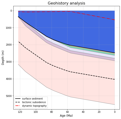
Geohistory analysis
The Geohistory Analysis notebook shows how to visualize the decompaction of stratigraphic layers of a drill site over time.
Note
The example notebooks are installed as part of the example data which can be installed by following these instructions.
Continental subsidence
One of the examples in that notebook demonstrates decompaction of a shallow continental drill site using backtracking. The tectonic subsidence (black dashed line) is from our model of continental subsidence and the paleo water depths (blue fill) are backtracked using tectonic subsidence and sediment decompaction. Note that, unlike backstripping, dynamic topography does affect tectonic subsidence (because its effects are included in the model of tectonic subsidence).
Note
There is a base sediment layer below the drill site (from the bottom of drill site to basement depth) since the drill site does not reach basement depth. And for this drill site the base sediment layer is quite thick because the default total sediment thickness grid is not as accurate near continental margins (compared to deeper ocean basins).
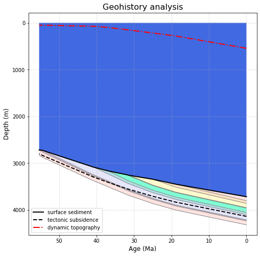
Oceanic subsidence
Another example in that notebook demonstrates decompaction of an oceanic drill site using backtracking. The tectonic subsidence (black dashed line) is from our model of oceanic subsidence and the paleo water depths (blue fill) are backtracked using tectonic subsidence and sediment decompaction. Note that, unlike backstripping, dynamic topography does affect tectonic subsidence (because its effects are included in the model of tectonic subsidence).
Note
There is a base sediment layer below the drill site (from the bottom of drill site to basement depth) since the drill site does not reach basement depth.