Paleobathymetry
Overview
The paleo_bathymetry module is used to generate paleo bathymetry grids by reconstructing and backtracking present-day sediment-covered crust through time.
PyBacktrack only generates paleobathymetry for crust that exists at present day. However you can optionally merge this with traditional paleobathymetry grids produced by an external workflow that generates paleobathymetry for synthetic crust. The traditional grids may contain paleobathymetry on subducted crust that is not covered by the reconstructed present-day sediment-deposited crust generated by pyBacktrack.
Running paleobathymetry
You can either run paleo_bathymetry as a built-in script, specifying parameters as command-line options (...):
python -m pybacktrack.paleo_bathymetry_cli ...
…or import pybacktrack into your own script, calling its functions and specifying parameters as function arguments (...):
import pybacktrack

pybacktrack.reconstruct_paleo_bathymetry_grids(...)
Note
You can run python -m pybacktrack.paleo_bathymetry_cli --help to see a description of all command-line options available, or
see the paleobathymetry reference section for documentation on the function parameters.
Example
To generate paleobathymetry NetCDF grids at 12 minute resolution from 0Ma to 240Ma in 1Myr increments, we can run it from the command-line as:
python -m pybacktrack.paleo_bathymetry_cli \
    -gm 12 \
    -ym M7 \
    -m GDH1 \
    --use_all_cpus \
    -- \
    240 paleo_bathymetry_12m_M7_GDH1
…where the -gm option specifies the grid spacing (12 minutes),
the -ym specifies the M7 dynamic topography model,
the -m option specifies the GDH1 oceanic subsidence model,
the --use_all_cpus option uses all CPUs (it also accepts an optional number of CPUs) and
the generated paleobathymetry grid files are named paleo_bathymetry_12m_M7_GDH1_<time>.nc.
…or write some Python code to do the same thing:
import pybacktrack

pybacktrack.reconstruct_paleo_bathymetry_grids(
    'paleo_bathymetry_12m_M7_GDH1',
    0.2,  # degrees (same as 12 minutes)
    240,
    dynamic_topography_model='M7',
    ocean_age_to_depth_model=pybacktrack.AGE_TO_DEPTH_MODEL_GDH1,
    use_all_cpus=True)  # can also be an integer (the number of CPUs to use)
Paleobathymetry output
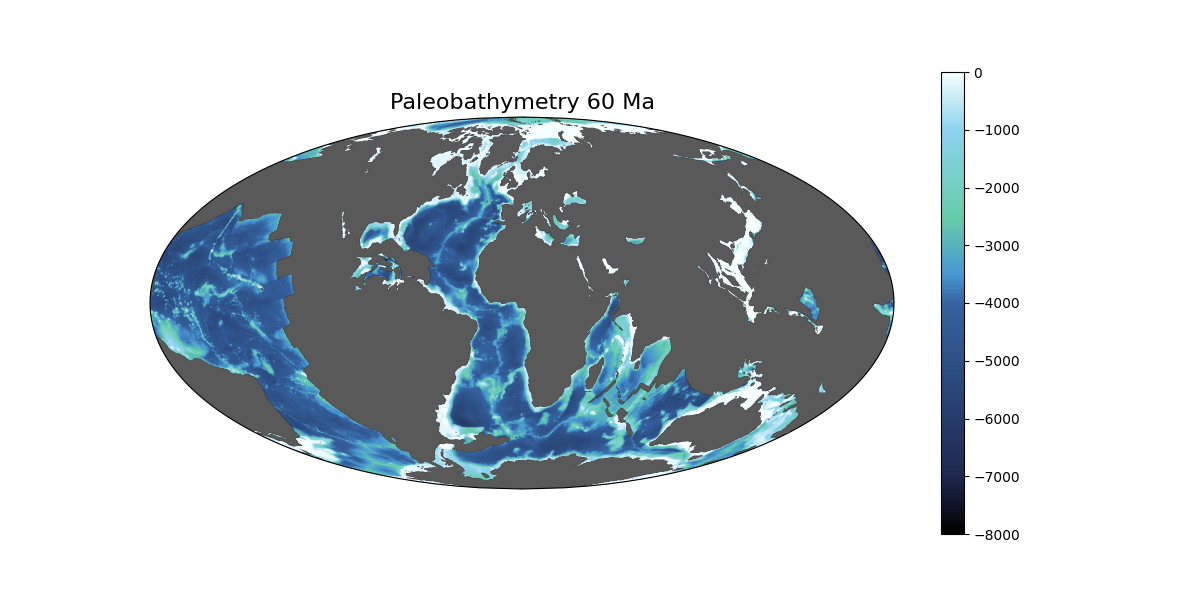
The following shows two of the 241 paleobathymetry NetCDF grids generated by the example above. The first at present day and the second at 60 Ma.

They were both generated using the Paleobathymetry notebook.
Note
The example notebooks are installed as part of the example data which can be installed by following these instructions.
Merging with traditional paleobathymetry
PyBacktrack only generates reconstructed paleobathymetry for sediment-deposited crust that exists at present day.
However you can merge this with traditional paleobathymetry grids produced by an external workflow that generates paleobathymetry for synthetic crust. This means the traditional grids will fill in paleobathymetry in regions where crust has been subducted at present day.
Note
This merging can be achieved using the --merge_paleo_bathymetry_filename_format command-line option
(or the merge_paleo_bathymetry_filename_format function argument of pybacktrack.reconstruct_paleo_bathymetry_grids).
Traditional paleobathymetry grids must still be produced by an external workflow. The notebooks Paleobathymetry and Reconstructing drill sites on paleobathymetry both merge traditional paleobathymetry created using Nicky Wright’s paleobathymetry workflow (currently in a private repository that might be incorporated into GPlately in the future).
There are traditional (and merged) paleobathymetry grids available for the default plate model in pyBacktrack (Zahirovic 2022) for both of its reference frames.
Traditional paleobathymetry for the Zahirovic 2022 plate model (for ages 0 to 410 Ma):
In the paleomagnetic reference frame (anchor plate 701701).
In the mantle reference frame (anchor plate 0).
And merged paleobathymetry for the Zahirovic 2022 plate model for ages 0 to 170 Ma (where 170 Ma is roughly when backtracked present-day crust no longer exists back in time):
In the paleomagnetic reference frame (anchor plate 701701).
In the mantle reference frame (anchor plate 0).
Note
The Alfonso 2024 plate model (ages 0 to 170 Ma) also has traditional and merged paleobathymetry grids available.
The following shows merged paleobathymetry in the paleomagnetic reference frame, at present day (0 Ma) and 60 Ma.
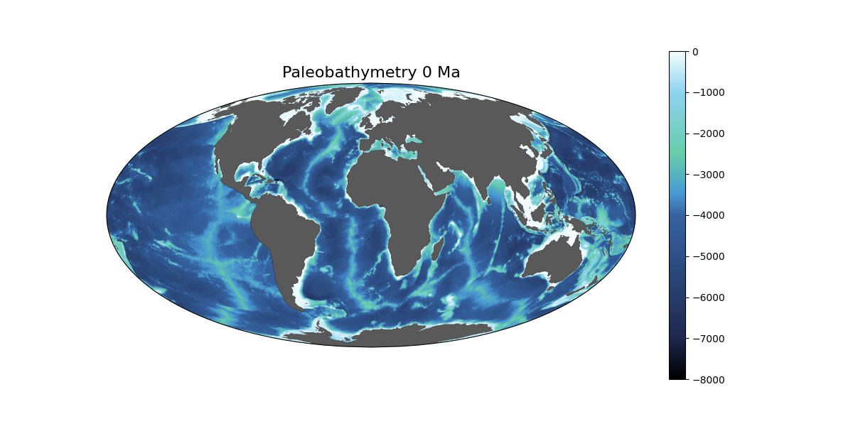
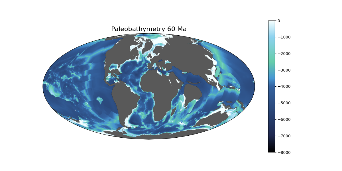
They were both generated using the Paleobathymetry notebook. Please see that notebook for details on how the merging was achieved.
Note the difference at 60 Ma in the merged paleobathymetry (compared to the unmerged paleobathymetry shown previously). For example, the region west of the Americas is now filled with traditional paleobathymetry. This region exists at 60 Ma but will be subducted at present day.
Hillshaded paleobathymetry
The above images show paleobathymetry with hillshading applied to display a 3D visualisation of the 2D bathymetry as if a directional light source was shining on it.
In those images (generated using the Paleobathymetry notebook)
the pyGMT function pygmt.grdgradient was used to compute directional derivatives from the paleobathymetry grid in the direction (azimuth) of a light source.
Assuming no ambient term, the directional derivatives are positive when the bathymetry slope is facing towards the light source (and negative when facing away).
These directional derivatives are then used to modify the RGB colours of the colour-mapped bathymetry to give a sense of shading from a directional light source.
Note
For pygmt.grdgradient, it is recommended to specify a gradient normalization using the cumulative Laplace distribution (eg, e0.5) instead of the cumulative Cauchy distribution (eg, t0.5)
as shown in the Paleobathymetry notebook.
Using the latter (Cauchy) distribution results in crisp hillshading at present day, but fades to indistinct shading at past geological times. This is because the former (Laplace) distribution puts the bulk of the gradient values within the flat part of the distribution whereas the latter (Cauchy) distribution puts them in the steep middle part. As we go back in geological time, the backtracked bathymetry (generated by pyBacktrack) is gradually replaced by traditional bathymetry. The backtracked bathymetry contains the higher detail of present-day bathymetry compared to traditional bathymetry. And so the change in gradient distribution from one time to the next results in less amplification when using the cumulative Laplace distribution (being in the flat part of the distribution). As a result the fade from crisp hillshading at present day to indistinct at past times is much less noticeable.
Paleobathymetry gridding procedure
Paleobathymetry gridding uses the built-in rift start/end age grids along with the existing subsidence models (continental rifting and oceanic) and the sediment decompaction functionality in pyBacktrack to generate paleo bathymetry grids (typically in 1 Myr intervals).
The paleo_bathymetry module has similar options to the backtrack module. Such as options for the present day grids containing age, bathymetry, crustal thickness and sediment thickness.
And options for the dynamic topography and sea level models. And the defaults for those options are the same as the backtrack module (except for the default lithology - see below).
For example, the paleo_bathymetry module defaults to the same present-day ETOPO1 bathymetry grid.
However the paleo_bathymetry module differs from the backtrack module in that, instead of a single point location for a drill site, a uniform grid of points containing sediment
(inside valid regions of the total sediment thickness grid) are backtracked to obtain gridded paleo water depths through time.
Note
Sediment grid points near trenches are excluded by default to avoid deep bathymetry areas near trenches appearing in the reconstructed grids.
Each trench has an exclusion distance on the subducting plate side (typically 60 kms) and an exlusion distance on the overriding plate side (typically 0 kms).
Any sediment grid points within these per-trench distances are excluded.
These distances are all built into pyBacktrack and vary from trench to trench.
They were hand tuned for each trench based on their resultant paleobathymetry.
However this masking near trenches can be removed by specifying --exclude_distances_to_trenches_kms 0 0
(for example, in the paleo bathymetry example above).
To retain the masking near trenches but remove the built-in hand tuning of distances you can specify --exclude_distances_to_trenches_kms 60 0.
This will apply a global exclusion distance of 60 kms on the subducting plate side (and no exclusion on the overriding plate side).
As with regular backtracking, those sediment grid points lying inside the age grid (valid regions) use an oceanic subsidence model and those outside use a continental rifting model. However, for the continental rifting model, in lieu of explicitly providing the rift start and end ages (as for a 1D drill site), each 2D grid point samples the built-in rift start/end age grids.
Note
You can optionally override the rift periods sampled from the built-in rift start/end grids with a single rift period using the --rifting_period command-line option.
However this overrides the spatially varying rift periods (of built-in rift start/end grids) with a constant rift period.
And hence is typically only useful for regional reconstructions (not global).
Each grid point is assigned a plate ID and reconstructed back through time (using a reconstruction model consisting of static polygons and rotations).
You can either use the default built-in reconstruction model, or specify your own static polygon and rotation files
(using the --static_polygon_filename and --rotation_filenames command-line options).
The default reconstruction model is Zahirovic 2022:
Zahirovic, S., Eleish, A., Doss, S., Pall, J., Cannon, J., Pistone, M., Tetley, M. G., Young, A., & Fox, P. (2022), Subduction kinematics and carbonate platform interactions. Geoscience Data Journal, 9(2), p.371-383, (data obtained here)
The default reference frame for the Zahirovic 2022 model is the mantle reference frame (anchor plate 0).
Alternatively you can use its paleomagnetic reference frame by specifying anchor plate 701701 (using the command-line option --anchor 701701).
This can be useful for paleoclimate-related research.
Note
In pyBacktrack versions 1.4 and older, the default reconstruction model was Müller 2019:
Müller, R. D., Zahirovic, S., Williams, S. E., Cannon, J., Seton, M., Bower, D. J., Tetley, M. G., Heine, C., Le Breton, E., Liu, S., Russell, S. H. J., Yang, T., Leonard, J., and Gurnis, M. (2019), A global plate model including lithospheric deformation along major rifts and orogens since the Triassic. Tectonics, vol. 38,.
1.5 onwards the default is Zahirovic 2022.701701).Note
Each grid point has a single lithology, with an initial compacted thickness sampled from the total sediment thickness grid at present day that is progressively decompacted back through geological time.
Note
The single lithology defaults to Average_ocean_floor_sediment which is the average of the ocean floor sediment.
This differs from the base lithology of drill sites where the undrilled portions of drill sites are usually below the
Carbonate Compensation Depth (CCD) where shale dominates. Note that you can override the default lithology by specifying the -b command-line option.
Note
In pyBacktrack versions 1.4 and older, the single lithology defaulted to Shale (not Average_ocean_floor_sediment).
The decompaction progresses incrementally (eg, in 1 Myr intervals) assuming a constant (average) decompacted sedimentation rate over the entire sedimentation period calculated as the fully decompacted initial thickness (ie, using surface porosity only) divided by the sedimentation period (from start of rifting for continental crust, and from crustal age for oceanic crust, to present day). Loading each reconstructed point’s decompacted thicknesses onto its modelled tectonic subsidence (oceanic or continental) back through time, along with the effects of dynamic topography and sea level models, reveals its history of water depths. Finally, the reconstructed locations of all grid points and their reconstructed bathymetries are combined, at each reconstruction time, to create a history of paleo bathymetry grids.
Note
You can optionally merge the paleobathymetry grids (produced by pybacktrack on present day crust) with externally-produced paleobathymetry grids (on synthetic crust).
This will insert paleobathymetry from the external grids only at grid locations not covered by the pybacktrack grids, after adding dynamic topography (if specified) to them.
This can be achieved using the --merge_paleo_bathymetry_filename_format command-line option.
Built-in rift gridding procedure
PyBacktrack comes with two built-in grids containing rift start and end ages on submerged continental crust at 5 minute resolution. This is used during paleobathymetry gridding to obtain the rift periods of gridded points on continental crust. It is also used during regular backtracking to obtain the rift period of a drill site on continental crust (when it is not specified in the drill site file or on the command-line).
The rift grids cover all submerged continental crust, not just those areas that have undergone rifting. Submerged continental crust is where the total sediment thickness grid contains valid values but the age grid does not (ie, submerged crust that is non oceanic).
The built-in rift grids were generated using the Zahirovic 2022 deforming plate model:
Zahirovic, S., Eleish, A., Doss, S., Pall, J., Cannon, J., Pistone, M., Tetley, M. G., Young, A., & Fox, P. (2022), Subduction kinematics and carbonate platform interactions. Geoscience Data Journal, 9(2), p.371-383, (data obtained here)
Note
In pyBacktrack versions 1.4 and older, the Müller 2019 deforming model was used to generate the built-in rift grids:
Müller, R. D., Zahirovic, S., Williams, S. E., Cannon, J., Seton, M., Bower, D. J., Tetley, M. G., Heine, C., Le Breton, E., Liu, S., Russell, S. H. J., Yang, T., Leonard, J., and Gurnis, M. (2019), A global plate model including lithospheric deformation along major rifts and orogens since the Triassic. Tectonics, vol. 38,.
Note
The rift grids were generated with pybacktrack/supplementary/generate_rift_grids.py.
This script can be obtained by installing the supplementary scripts.
The following paragraph gives a brief overview of rift gridding…
First, grid points on continental crust that have undergone extensional deformation (rifting) during their most recent deformation period have their rift start and end ages assigned as the start and end of that most recent deformation period (for each grid point). Next, grid points on continental crust that have undergone contractional deformation during their most recent deformation period have their rift periods set to default values (currently 200 to 0 Ma) to model these complex areas with simple rifting (despite a rifting model no longer strictly applying). So that covers the deforming grid points on continental crust. Next, the non-deforming grid points on continental crust obtain their rift period from the nearest deforming grid points. This ensures that all continental crust contains a rift period and hence can be used to generate paleobathymetry grids from all present day continental crust.
Note
1.4 and older, only the continental grid points that were submerged were stored in the built-in rift grids,
since only submerged crust needs backtracking.1.5 onwards, the built-in rift grids have global coverage.
Here each grid point that is not on deforming continental crust (ie, could be oceanic or non-deforming continental) inherits the rift period of the nearest grid point on deforming continental crust.
In submerged continental regions, the rift periods are the same as in pyBacktrack 1.4, but we now also get rift periods outside submerged continental regions.
This avoids tying the built-in rift grids to the default age grid (determines which crust is continental) and the default total sediment thickness grid (determines which crust is submerged).
For example, you might specify an age grid that has a slightly different continental-oceanic boundary.
Or you might specify a total sediment thickness that has a slightly different coastline.
And in these cases you can now generate paleobathymetry grids that don’t have gaps due to misalignments between, for example, your age grid boundary and the built-in rift grid boundaries (which are now boundaryless).The following paragraph gives a more detailed explanation of how deformation in particular is used in pybacktrack/supplementary/generate_rift_grids.py…
The script allows one to specify a total sediment thickness grid and an age grid (defaulting to those included with pyBacktrack). Grid points are uniformly generated in longitude/latitude space on continental crust. Next pyGPlates is used to load the Zahirovic 2022 topological plate model (containing rigid plate polygons and deforming networks) and reconstruct these continental grid points on back through geological time. Note that plate IDs do not need to be explicitly assigned in order to be able to reconstruct because functionality in pyGPlates, known as reconstructing by topologies, essentially continually assigns plate IDs using the topological plate polygons and deforming networks while each grid point is reconstructed back through time. This ensures the path of each grid point is correctly reconstructed through deforming regions so that we can correctly determine when it enters and exits a deforming region. During this reconstruction each grid point is queried (at 1Myr intervals) whether it passes through a deforming network. The time at which a reconstructed grid point first encounters a deforming network (going backward in time) becomes its potential rift end time. Following that point further back in time we find when it first exits a deforming network (again going backward in time), which becomes its potential rift start time. We also keep track of a crustal stretching factor through time for each grid point so we can distinguish between extensional and contractional deformation.